Optimization module usage
This guide explains how to assemble an optimization run. The
examples/simple_biaxial_fit.py script is an illustration, but the focus here is
on the structure so you can swap in your own templates, data, and adapters.
Objective (what is minimized)
Default cost: least squares over cases/experiments
\(\theta\): parameters from
ParameterSpace.\(f_{c,e}(\theta)\): simulated response from the adapter (reads
.xpltviaxpltand can slice any view).\(y_{c,e}\): experimental data (
ExperimentSeries).\(w_{c,e}\): optional weights per case/experiment.
Reparameterization (OptimizerOptions.reparametrize) maps bounded parameters to
an unbounded internal space for stability. Jacobians (JacobianOptions.enabled)
are finite-difference approximations of \(\partial f / \partial \theta\).
Overview (roles and features)
ExperimentSeries: measured data (
x,y) for the objective.ParameterSpace: parameters, initial guesses, bounds, optional
xi.FebTemplate + ParameterBinding: point to a
.febtemplate and bind parameter names to XML paths.SimulationAdapter: callable that opens
.xpltwithxplt, slices views, and returns arrays for the objective (any view slicing works).SimulationCase: groups template, experiments, adapters, grid policy, and runtime settings (subfolder, threads).
EngineOptions: knobs for jacobian, cleanup, runner, storage, monitor, optimizer.
Engine: schedules FEBio runs (parallel if requested), collects adapter outputs, and drives the optimizer.
Assembly flow
data → ExperimentSeries
parameters → ParameterSpace
template + bindings → FebTemplate/ParameterBinding
template + experiments + adapters + grid → SimulationCase(s)
options → EngineOptions
Engine(ParameterSpace, cases, options) → run() → optimized θ
Adapter structure (xplt in action)
def read_sigma_xx(xplt_path):
    xp = xplt(str(xplt_path))
    xp.readAllStates()
    stress = xp.results["stress"].domain("volume")
    sigma_xx = stress.time(":").items(9).comp("xx")
    times = np.asarray(xp._time, dtype=float)
    return times, np.asarray(sigma_xx, dtype=float)
Adapters are plain callables: slice nodesets, surfaces, enodes, or components by name, and post-process before returning arrays.
Assembling your own run (steps)
Load experiment data:
exp_data = np.loadtxt(DATA_PATH)
exp_series = ExperimentSeries(x=exp_data[:, 0], y=exp_data[:, 1])
Define parameters and bounds:
parameter_space = ParameterSpace(xi=2.0)
parameter_space.add_parameter(name="G", theta0=0.6, bounds=(0, 10))
Create template and bindings:
template = FebTemplate(
    TEMPLATE_PATH,
    bindings=[ParameterBinding(theta_name="G", xpath=".//Material/material[@id='1']/G")],
)

# For more flexible writes, one fitted parameter can drive multiple FEB nodes.
# Example: one angle "phi" controlling mirrored fiber vectors.
import math

template = FebTemplate(
    TEMPLATE_PATH,
    bindings=[
        EvaluationBinding(
            xpath=".//Material/material[@id='1']/solid[2]//fiber/vector",
            value=lambda th: (
                f"{math.cos(th['phi']):.6f},0,{math.sin(th['phi']):.6f}"
            ),
        ),
        EvaluationBinding(
            xpath=".//Material/material[@id='1']/solid[3]//fiber/vector",
            value=lambda th: (
                f"{math.cos(th['phi']):.6f},0,{-math.sin(th['phi']):.6f}"
            ),
        ),
    ],
)
Build one or more cases:
case = SimulationCase(
    template=template,
    subfolder="biaxial",
    experiments={"biax1": exp_series},
    adapters={"biax1": SimulationAdapter(read_sigma_xx)},
    omp_threads=5,
    grids={"biax1": GridPolicyOptions(policy="fixed_user", values=FIXED_GRID.tolist())},
)
Configure EngineOptions and run:
options = EngineOptions(
    jacobian=JacobianOptions(enabled=True, perturbation=1e-3, parallel=True),
    cleanup=CleanupOptions(remove_previous=True, mode="all"),
    runner=RunnerOptions(jobs=PARALLEL_JOBS, command=FEBIO_COMMAND),
    storage=StorageOptions(mode="tmp", root=WORK_ROOT),
    monitor=MonitorOptions(enabled=True),
    optimizer=OptimizerOptions(
        name="least_squares",
        settings={"ftol": 1e-6, "xtol": 1e-6},
        reparametrize=True,
    ),
)

engine = Engine(parameter_space=parameter_space, cases=[case], options=options)
result = engine.run()
Capabilities (engine)
Multiple cases: fit several datasets simultaneously.
Parallel runs:
RunnerOptions.jobscontrols concurrency; combine withJacobianOptions.parallelfor concurrent Jacobian entries.Grid policies: per-case
GridPolicyOptions(fixed_user or other strategies).Cleanup: remove or keep old runs via
CleanupOptions.Storage: temporary or disk-backed run trees via
StorageOptions.Monitoring/logs: live monitor plus final artifacts (generated
.feb,.xplt, FEBio stdout/stderr) for the optimizer’s final result.Optimizers: choose backend and pass settings; enable reparameterization for bounded problems.
EngineOptions in depth
JacobianOptions
enabled: finite-difference Jacobian on/off; required for gradient-based optimizers or sensitivities.perturbation: finite-difference step size (accuracy vs. noise trade-off).parallel: compute Jacobian columns concurrently (each perturbation is a FEBio run).
CleanupOptions
remove_previous: delete older transient evaluation folders during the run.mode:"none"keeps transient evaluation folders for debugging;"all"removes them after final artifacts are exported.
RunnerOptions
jobs: max concurrent FEBio runs (throughput vs. CPU/RAM use).command: how to invoke FEBio, e.g.,("febio4", "-i"); adjust for MPI or extra flags.
StorageOptions
mode:"tmp"runs simulations in temporary storage;"disk"runs them underroot.root: work directory foroptimization.log,results/curve exports, andoptimized_simulations/final FEBio outputs.
MonitorOptions
enabled: toggle live monitoring/log streaming; when enabled, progress is pushed as runs finish.url: optional monitor web URL shown in startup logs; defaults tohttp://127.0.0.1:8765when omitted.
OptimizerOptions
name: optimizer backend (e.g.,"least_squares","minimize","differential_evolution").settings: forwarded to the optimizer (tolerances, max iterations, damping/ line search controls, etc.).reparametrize: transform bounded parameters to unbounded space internally.
"differential_evolution"wraps SciPy’s global optimizer and requires finite bounds for all varying parameters. Itssettings["workers"]option uses a pyfebiopt-managed thread pool, not SciPy’s default multiprocessing pool, so FEBio subprocess evaluations can run concurrently without pickling the engine state. Whenworkers > 1, pyfebiopt forcesupdating="deferred"and reports one progress row per generation. Size resources carefully: total FEBio concurrency is approximatelyworkers * RunnerOptions.jobs * number_of_cases. For expensive FEBio runs, start withpolish=FalseandRunnerOptions.jobs=1when enabling differential-evolution workers.
Monitoring and logging
Live monitor: enable via
MonitorOptions.enabled. A lightweight service streams run status (case, iteration, parameters, objective). Point your browser to the monitor endpoint to watch progress in near real-time.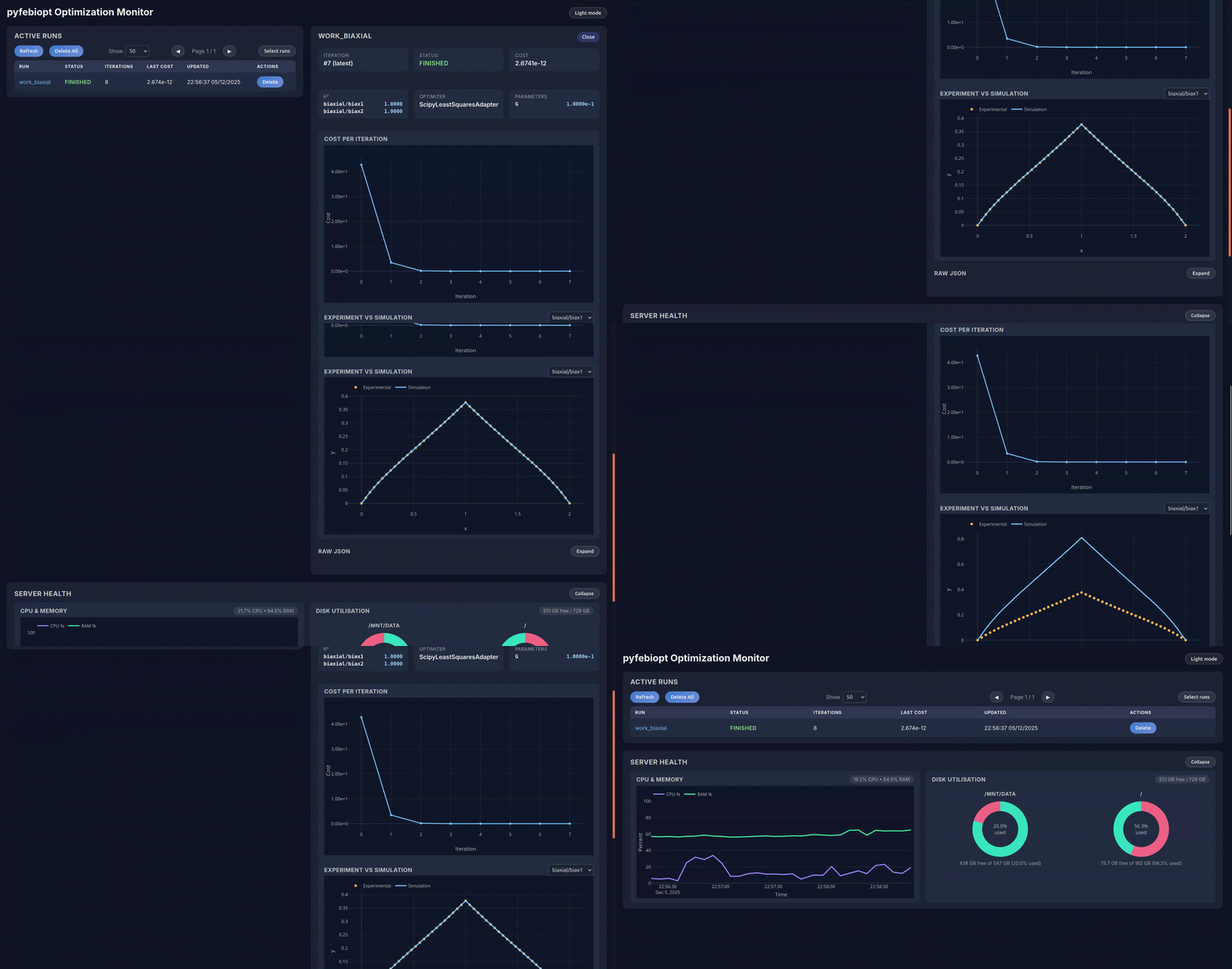
Logs/artifacts: the work folder contains
optimization.log,results/*.txtcurve exports, andoptimized_simulations/with final.feb,.xplt, and FEBio log files.Cleanup:
CleanupOptionscontrols transient evaluation folders only; exported final artifacts are preserved.
Assembly checklist
Prepare experiment data (
ExperimentSeries).Define
ParameterSpacewith initial guesses and bounds.Set up FEB template + parameter bindings.
Write adapters that read
.xpltviaxpltand return arrays.Create one or more
SimulationCaseobjects (template, experiments, adapters, grids, runtime knobs).Configure
EngineOptions(jacobian, cleanup, runner, storage, monitor, optimizer).Instantiate
Engineand callrun().